Long run is that time period when a firm can change all its inputs. In fact, there are no fixed inputs in the long run; all inputs are variable. Thus, in the long run, there is no fixed cost; all costs are variable. That is why, in the long run, a firm can change its scale of production according to its needs.
In the short run, size of a plant or the scale remains fixed while, in the long run, changes in plant size can be made. In the long run, a firm can move from one plant to another plant thereby giving rise to different cost relationships. If the situation demands, it can build up a large- sized plant or a smaller one.
It is to be mentioned here that long run is a “planning horizon” in the sense that it acts as a guide to the firm relating to the future output decision. We know that production takes place in the short run. In brief, short run is the ‘operating period’ of a firm. Every firm aims at production for a future date and chooses many aspects of the short run situations among which the firm may choose.
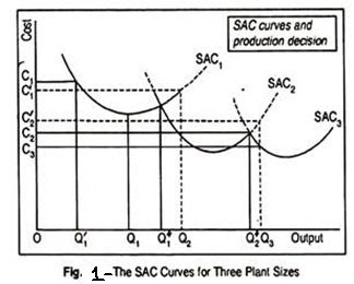
LAC is, thus, derived from the SAC curves. LAC depicts the lowest possible average cost for producing various possible levels of output. To derive the LAC curve, we assume that there are three different sizes of plants in an industry— small, medium and large. Small-sized, medium-sized, and large- sized plants are represented by the three SAC curves—SAC1, SAC2 and SAC3, respectively, as shown in Fig. 1.

These SAC curves are also called plant curves. Since we are considering the long run situation, the firm can choose any plant size in which it will operate in the future to produce a given output level at the lowest possible cost.
If the firm decides to produce OQ1, it will choose plant size denoted by SAC1. A lower output (say OQ’1) can also be produced on SAC1 but at a higher cost. But the same plant size, i.e., SAC1 enables a firm to produce large output at a lower cost. If OQ2 is considered to be most profitable level output, the firm will select SAC2 —the medium-sized plant.
It will select the large-sized plant, SAC3, to produce OQ3 level of output. But taking such decision is not an easy job as it appears at first sight. Suppose, the firm operates at SAC1 and demand for its product gradually rises. Of course, it can produce OQ1 at the lowest cost even operating on SAC1. Production beyond OQ1 will entail a larger cost.
If the firm expects to produce OQ”1, (as in Fig. 2) its choice of plant size becomes a difficult one since costs are the same for both the plant-sizes—SAC1 and SAC2. Now the choice of the optimal plant size depends on the firm’s anticipation or expectation regarding its demand for product in the coming years. At this level of output, cost cannot be the determinant of the choice of a plant size.
It is quite natural that the firm expects its demand for the product to increase in future. So, the firm, quite likely, will install the plant number SAC2 rather than SAC1. Larger outputs can now be produced with lower cost. Similarly, though output OQ”2 can be produced by both the plant sizes, SAC2 and SAC3, it is better to use the plant size represented by SAC3 since larger output (OQ3) can be produced at a lower cost (OQ3).
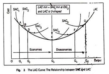
However, let us assume that the industry faces a large number of plant sizes represented by, say, five SAC curves, as shown in Fig.2. These curves will generate a smooth and continuous curve called the ‘planning curve’ or the LAC curve.

Each point on this curve shows the least possible cost for producing the corresponding level of output. The LAC curve is a planning curve because it is the curve which helps a firm to decide which plant is to be established in order to produce an output level consistent with the optimal cost.
The firm selects that short run plant which yields the minimum cost of producing the anticipated output level. To produce a particular output in the long run, the firm must select a point on the LAC curve corresponding to that output, and it will then build a relevant short run plant and operate on the corresponding SAC curve.
Suppose, the firm thinks that for producing output OQ1 point A on SAC1 becomes the most profitable one. It will then build up a plant at the lower cost represented by the curve SAC1. [At point A, the SAC1 curve is tangent to the LAC curve.] However, the firm could reduce its cost by expanding output to the amount associated with point B, the minimum point on the SAC1 curve.
But the firm anticipates that demand for its product in future would be rising. So, it would construct a new plant, represented by the SAC2 curve and will operate at point D on the SAC2 curve, thereby lowering its unit cost and not on the lowest point on the SAC2 curve [Corresponding to the output level OQ2, SAC2 is tangent to the curve LAC].
Similarly, for output OQ3, the firm would construct SAC3 plant and operate at E where unit costs become the lowest. [Again, SAC3 is tangent to the LAC curve] Same would be the case for all other outputs in the long run. For output OQ4, the firm would construct plant size SAC4 and would operate at point F.
However, the minimum point of SAC now lies to the left of the operational point, F. Similarly, OQ5 output could be produced by the plant size SAC5.
The firm should operate at point G on the curve SAC5. Each point of the LAC curve is, thus, the point of tangency with the corresponding SAC curves. The LAC curve is the locus of all the tangency points. As a consequence of this, the LAC curve is called the ‘envelope curve’ as it envelops or supports a family of SAC curves.
It is to be remembered here that the LAC curve, throughout its length, is not tangential to the minimum points of all the SAC curves. When LAC is falling, it is tangential to the falling portion of the SAC curves, not to the minimum point of the SAC curves.
For instance, the firm operates at point A on the curve SAC, the falling portion, rather than B where costs are the lowest. In other words, since the slope of the LAC curve up to point E is negative, the slope of the SAC curves must also be negative. This is because, at the tangency points, both the SAC and LAC curves have the same slopes. Only at point E, the minimum point of LAC is tangent to the minimum point of the SAC.
To the right of this point, as LAC is rising, it is tangent to the rising portion of SAC curves. Note that, at the points of tangency, SAC = LAC, but to the right or left of the tangency point SAC > LAC. However, the minimum points of SAC curves below OQ3 output lie to the right of the operational point. Beyond OQ3 output, SAC’s minimum points lie to the left of the operational point.
Thus, we can say that the LAC curve is U-shaped—it first falls, reaches minimum, and rises afterwards as output expands. But the U-shape of the LAC curve is less pronounced than the U-shape of SAC curve.
One thought on “Long Run Average Cost (LAC)”