Valuation of Options Contract

In finance, a price (premium) is paid or received for purchasing or selling options.

The value of an option can be estimated using a variety of quantitative techniques based on the concept of risk neutral pricing and using stochastic calculus. In general, standard option valuation models depend on the following factors:

• The current market price of the underlying security
• The strike price of the option, particularly in relation to the current market price of the underlying asset (in the money vs. out of the money)
• The cost of holding a position in the underlying security, including interest and dividends
• The time to expiration together with any restrictions on when exercise may occur, and
• An estimate of the future volatility of the underlying security’s price over the life of the option.

Binomial Option Pricing Model

The simplest method to price the options is to use a binomial option pricing model. This model uses the assumption of perfectly efficient markets. Under this assumption, the model can price the option at each point of a specified time frame.

Under the binomial model, we consider that the price of the underlying asset will either go up or down in the period. Given the possible prices of the underlying asset and the strike price of an option, we can calculate the payoff of the option under these scenarios, then discount these payoffs and find the value of that option as of today.

Figure 1. Two-period binomial tree

Black-Scholes Model

The Black-Scholes model is another commonly used option pricing model. This model was discovered in 1973 by the economists Fischer Black and Myron Scholes. Both Black and Scholes received the Nobel Memorial Prize in economics for their discovery.

The Black-Scholes model was developed mainly for pricing European options on stocks. The model operates under certain assumptions regarding the distribution of the stock price and the economic environment. The assumptions about the stock price distribution include:

• Continuously compounded returns on the stock are normally distributed and independent over time.
• The volatility of continuously compounded returns is known and constant.
• Future dividends are known (as a dollar amount or as a fixed dividend yield).

The assumptions about the economic environment are:

• The risk-free rate is known and constant.
• There are no transaction costs or taxes.
• It is possible to short-sell with no cost and to borrow at the risk-free rate.

Nevertheless, these assumptions can be relaxed and adjusted for special circumstances if necessary. In addition, we could easily use this model to price options on assets other than stocks (currencies, futures).

 The main variables used in the Black-Scholes model include:

• Price of underlying asset (S) is a current market price of the asset
• Strike price (K) is a price at which an option can be exercised
• Volatility (σ) is a measure of how much the security prices will move in the subsequent periods. Volatility is the trickiest input in the option pricing model as the historical volatility is not the most reliable input for this model
• Time until expiration (T) is the time between calculation and an option’s exercise date
• Interest rate (r) is a risk-free interest rate
• Dividend yield (δ) was not originally the main input into the model. The original Black-Scholes model was developed for pricing options on non-paying dividends stocks.

From the Black-Scholes model, we can derive the following mathematical formulas to calculate the fair value of the European calls and puts:

The formulas above use the risk-adjusted probabilities. N(d₁) is the risk-adjusted probability of receiving the stock at the expiration of the option contingent upon the option finishing in the money. N(d₂) is the risk-adjusted probability that the option will be exercised. These probabilities are calculated using the normal cumulative distribution of factors d₁ and d₂.

The Black-Scholes model is mainly used to calculate the theoretical value of European-style options and it cannot be applied to the American-style options due to their feature to be exercised before the maturity date.

Monte-Carlo Simulation

Monte-Carlo simulation is another option pricing model we will consider. The Monte-Carlo simulation is a more sophisticated method to value options. In this method, we simulate the possible future stock prices and then use them to find the discounted expected option payoffs.

In this article, we will discuss two scenarios: simulation in the binomial model with many periods and simulation in continuous time.

Scenario 1

Under the binomial model, we consider the variants when the asset (stock) price either goes up or down. In the simulation, our first step is determining the growth shocks of the stock price. This can be done through the following formulas:

h in these formulas is the length of a period and h = T/N and N is a number of periods.

After finding future asset prices for all required periods, we will find the payoff of the option and discount this payoff to the present value. We need to repeat the previous steps several times to get more precise results and then average all present values found to find the fair value of the option.

Scenario 2

In the continuous time, there is an infinite number of time points between two points in time. Therefore, each variable carries a particular value at each point in time.

Under this scenario, we will use the Geometric Brownian Motion of the stock price which implies that the stock follows a random walk. Random walk means that the future stock prices cannot be predicted by the historical trends because the price changes are independent of each other.

In the Geometric Brownian Motion model, we can specify the formula for stock price change:

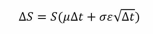
Where:

S – stock price

ΔS – change in stock price

µ – expected return

t – time

σ – standard deviation of stock returns

↋ – random variable µ 

Unlike the simulation in a binomial model, in continuous time simulation, we do not need to simulate the stock price in each period, but we need to determine the stock price at the maturity, S(T), using the following formula:

We generate the random number ↋ and solve for S(T). Afterward, the process is similar to what we did for simulation in the binomial model: find the option’s payoff at the maturity and discount it to the present value.