Measurement of Beta

The beta (β) of an investment security (i.e. a stock) is a measurement of its volatility of returns relative to the entire market. It is used as a measure of risk and is an integral part of the Capital Asset Pricing Model (CAPM). A company with a higher beta has greater risk and also greater expected returns.

The beta coefficient can be interpreted as follows:

• β =1 exactly as volatile as the market
• β >1 more volatile than the market
• β <1>0 less volatile than the market
• β =0 uncorrelated to the market
• β <0 negatively correlated to the market

Examples of beta

High β: A company with a β that’s greater than 1 is more volatile than the market. For example, a high-risk technology company with a β of 1.75 would have returned 175% of what the market return in a given period (typically measured weekly).

Low β: A company with a β that’s lower than 1 is less volatile than the whole market. As an example, consider an electric utility company with a β of 0.45, which would have returned only 45% of what the market returned in a given period.

Negative β: A company with a negative β is negatively correlated to the returns of the market. For an example, a gold company with a β of -0.2, which would have returned -2% when the market was up 10%.

Equity Beta and Asset Beta

Levered beta, also known as equity beta or stock beta, is the volatility of returns for a stock taking into account the impact of the company’s leverage from its capital structure. It compares the volatility (risk) of a levered company to the risk of the market.

Levered beta includes both business risk and the risk that comes from taking on debt. It is also commonly referred to as “equity beta” because it is the volatility of an equity based on its capital structure.

Asset beta, or unlevered beta, on the other hand, only shows the risk of an unlevered company relative to the market. It includes business risk but does not include leverage risk.

Project Beta

For simplicity throughout previous chapters we have used a general beta factor (b) applicable to the overall systemic risk of portfolios, securities and projects. But now our analysis is becoming more focused, precise notation and definitions are necessary to discriminate between systemic business and financial risk. Table 7.1 summarizes the beta measures that we shall be using for future reference and also highlights a number of problems.

b = total systematic risk, which relates portfolio, security and project risk to market risk.

b = the business risk of a specific project (project risk) for investment appraisal.

bf = the published equity beta for a company that incorporates business risk and systematic financial risk if the firm is geared.

bA = the overall business risk of a firm’s assets (projects). It also equals a company’s

deleveraged published beta (bf) which measures business risk free from financial risk.

bD = the beta value of debt (which obviously equals zero if it is risk-free).

bf„ and bfG are the respective equity betas for similar all-share and geared companies.

When an all-equity company is considering a new project with the same level of risk as its current portfolio of investments, total systematic risk equals business risk, such that:

When a company is funded by a combination of debt and equity, this series of equalities must be modified to incorporate a premium for systematic financial risk. As we shall discover, the equity beta (bE) will be a geared beta reflecting business risk plus financial risk, which measures shareholder exposure to debt in their firm’s capital structure. Thus, the equity beta of an all-share company is always lower than that for a geared firm with the same business risk.

Irrespective of a gearing problem, Table 7.1 reveals a further weakness of the CAPM. A company’s asset beta (bA) should produce a discount rate that is appropriate for evaluating projects with the same overall risk as the company itself. But what if a new project does not reflect the average risk of the company’s assets? Then the use of bA is no more likely to produce a correct investment decision than the use of a WACC calculation.

To illustrate the point, Figure 7.1 graphs the Security Market Line (SML) to show the required return on a project for different beta factors, with a company’s WACC. The use of the overall cost of capital to evaluate projects whose risk differs from the company’s average will be sub-optimal where the IRR of the project is in either of the two shaded sections. To calculate the correct CAPM discount rate using Equation (45), we must determine the project beta.

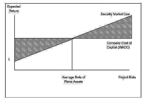
Figure 7.1: The SML, WACC and Project Betas

The company’s average beta, shown in the diagram, provides a measure of risk for the firm’s overall returns compared with that of the market. However, management’s investment decision is whether or not to invest in a project. So, like the WACC, if the project involves diversification away from the firm’s core activities, we must use a beta coefficient appropriate to that class of investment. The situation is similar to a stock market investor considering whether to purchase the shares of the company. The individual would need to evaluate the share’s return by using the market beta in the CAPM.

Even if diversification is not contemplated, the project’s beta factor may not conform to the average for the firm’s assets. For example, the investment proposal may exhibit high operational gearing (the proportion of fixed to variable costs) in which case the project’s beta will exceed the average for existing operations.

A serious conflict (the agency problem) can also arise for those companies producing few products, or worse still a single product, particularly if management approach their capital budgeting decisions based on self-interest and short-termism, rather than shareholder preferences. Shareholders with well-diversified corporate holdings who dominate such companies may prefer to see projects with high risk (high beta coefficients) to balance their own portfolios. Such a strategy may carry the very real threat of bankruptcy but in the event may have very little impact their overall returns. For corporate management, the firm’s employees and its suppliers, however, the policy may be economic suicide.

Fortunately, if a beta is required to validate the CAPM for project appraisal, help is at hand. Management can obtain factors for companies operating in similar areas to the proposed project by subscribing to the many commercial services that regularly publish beta coefficients for a large number of companies, world wide. Their listings also include stock exchange classifications for industry betas. These are calculated by taking the market average for quoted companies in the same industry. Research reveals that the measurement errors of individual betas cancel out when industry betas are used. Moreover, the larger the number of comparable beta constituents, the more reliable the industry factor.

So, if management wish to obtain an estimate for a project’s beta, it can identify the industry in which the project falls, and use that industry’s beta as the project’s beta. This approach is particularly suitable for highly diversified and divisionalised companies because their WACC or market beta would be of little relevance as a discount rate for its divisional operations.

As an alternative to stock market data, management can also estimate a project’s beta from first principles by calculating its F-value.

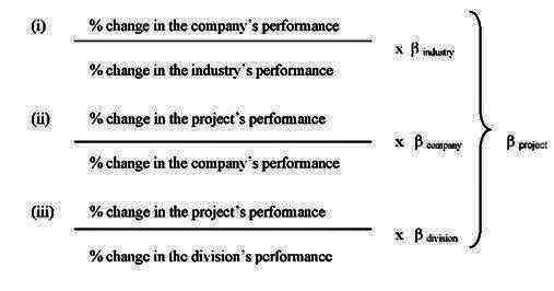
The F-value of a project is rather like a beta factor in that it measures the variability of a project’s performance, relative to the performance of an entity for which a beta value exists.

The entity could be the industry in which the project falls, the firm undertaking the project, or a division within the firm that is responsible for the project.

A project’s F-value is defined as follows:

As a result, we can obtain an estimate of a project’s beta through one of three routes:

Portfolio Beta

Calculating the volatility, or beta, of your stock portfolio is probably easier than you think. A beta of 1 means that a portfolio’s volatility matches up exactly with the markets. A higher beta indicates great volatility, and a lower beta indicates less volatility. To do it, you’ll need to know the percentage of your portfolio by individual stock and the beta for each of those stocks.

The first step is to multiply the percentage of your portfolio and the beta for each individual stock. Once that is done, simply add up the results and you’ll have your portfolio beta.

This method is a simple weighted average calculation. It’s an easy way to quickly assess your entire portfolio’s volatility. It only works though if the individual stock’s betas are calculated correctly and comparably. Using a six month time period to calculate one stocks beta and a six year period to calculate the other will give you a much different result than using the same time period across the board. Likewise, it’s wise to use the same index for each individual stock’s beta so that your portfolio beta will have consistency with that index as well. For most portfolios, the S&P 500 is a reasonable index to start with.

It’s not required to use the same time period and index for each stock, but it is important to understand how differences in each individual stock’s beta will impact the result for your entire portfolio.