Consumption function, Investment function

In economics, the consumption function describes a relationship between consumption and disposable income. The concept is believed to have been introduced into macroeconomics by John Maynard Keynes in 1936, who used it to develop the notion of a government spending multiplier.

The Keynesian consumption function expresses the level of consumer spending depending on three factors.

• Yd = disposable income (income after government intervention – e.g. benefits, and taxes)
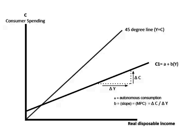
• a = autonomous consumption (consumption when income is zero. e.g. even with no income, you may borrow to be able to buy food)
• b = marginal propensity to consume (the % of extra income that is spent). Also known as induced consumption.

Consumption function formula

    C = a + b Yd

This suggests consumption is primarily determined by the level of disposable income (Yd). Higher Yd leads to higher consumer spending.

This model suggests that as income rises, consumer spending will rise. However, spending will increase at a lower rate than income.

• At low incomes, people will spend a high proportion of their income. The average propensity to consume could be one or greater than one. This means people spend everything they have. When you have low income, you don’t have the luxury of being able to save. You need to spend everything you have on essentials.
• However, as incomes rise, people can afford the luxury of saving a higher proportion of their income. Therefore, as incomes rise, spending increases at a lower rate than disposable income. People with high incomes have a lower average propensity to spend.

Limitations of consumption function

• Life cycle factors, Students more likely to borrow and spend during university days.
• Behavioural factors, People may be influenced by general optimism.

importance of the concept of propensity to consume is that we derive the theory of multiplier from it which has great practical importance in the formulation of macro-economic policy, especially of public works in times of depression. The magnitude of multiplier is equal to the reciprocal of one minus marginal propensity to consume (K = 1/1-MPC) where K stands for multiplier and MPC for marginal propensity to consume. According to this concept of multiplier, when investment increases, in­come, output and employment increase by a multiple amount, depending upon the size of the multiplier.

Income increases manifold than the original investment because of the nature of consumption function. When some investment in some projects is undertaken, it leads to the increase in income of those employed in the projects but the process does not stop here.

The increases in income are further spent on consumption and this leads to further increase in income and so the chain of increases in income and consumption continues and the ultimate increase in income and employment is multiple of the original increment in investment.

If the marginal propensity to consume were equal to zero, then all increments in income brought about by additional investment would have been saved and therefore multiplier process would not have worked. Since the marginal propensity to consume is greater than zero, the increase in net investment has a multiplier effect on income, output and employment. Thus, the effect of investment on income depends on the size of the multiplier which depends on the value of the marginal propensity to consume. The greater the marginal propensity to consume, the greater the size of the multiplier.

(4) From the concept of consumption function, we can also explain why there is a tendency for the marginal efficiency of capital to decline. The declining tendency of the marginal effi­ciency of capital is due to the nature of the consumption function. Two features of consumption function are important. First, the marginal propensity to consume is less than one which implies that as income increases, consumption increases less than this. Secondly, consumption function is stable in the short run i.e., it does not shift much in the short run.

As we know that the level of investment is a crucial factor in the determination of income and employment, fluctuations in the levels of income and employment depend primarily on the fluctuations in investment. The investment demand in the short run is determined by the rate of interest on the one hand and marginal efficiency of capital on the other. Since the rate of interest is relatively sticky, it is the marginal efficiency of capital which greatly affects the level of investment in the short run.

Marginal efficiency of capital is nothing but the expected rate of profit on investment in the future. Thus, the marginal efficiency of capital is determined by the expectations of the entrepreneurs regarding the earning of profits from capital assets in the future.

Now, the most, important fact that affects the entrepreneurs expectations regarding profit prospects and thereby the marginal efficiency of capital is the level of future consumption demand for goods and services. Their estimate of future consumption demand depends on, among others, on the population growth. If population growth of a country is expected to fall as was estimated in the early thirties when Keynes wrote his book (General Theory of Employment, Interest and Money), this would adversely affect future consumption demand which in turn would adversely affect investment in the long run, Besides, according to Keynes, average propensity to consume (APC) falls as income of a community increases overtime.

This also adversely affects inducement to invest. If there does not occur capital-using technological change, this will result in decline in investment opportunities in the long run, causing secular stagnation. Thus, we see that in the Keynesian scheme of things level of investment depends upon the level of consumption demand in the long run.

Since marginal propensity to consume is less than one and also the consumption function is stable when income increases, consumption does not increase proportionately. As a result, the aggregate demand becomes deficient and the marginal efficiency of capital declines. The decline in the marginal efficiency of capital adversely affects investment which stops rising. As a result, the growth process stops and economic recession occurs.

In this way, Keynes himself and later important Keynesian economist, Prof. A.H. Hansen developed the theory of secular stagnation for the mature capitalist economies. This secular stagnation theory is based upon the assertion that investment opportunities in a capitalist economy will be exhausted soon due to the absence of the possibilities of increasing consumption demand. The meagre possibilities of increasing investment in the mature capitalist economies, according to them, were partly due to the constancy of consumption function and declining average propensity to consume which caused the marginal efficiency of capital to decline.

Theory of secular stagnation has not been found true by empirical evidence in the last over seventy years of growth in the capitalist developed countries. However, the fact that current consumption is influenced by changes in rate of interest, stock of wealth and price level and further that it is the changes current consumption level that determine short-run business expectations about future yields from investment which cause fluctuations in investment.

Together with the working of multiplier fluctuations in investment cause business cycles in a free market economy. This shows the great importance of Keynes’s consumption function and the factors that determine it.

Investment function

The investment function is a summary of the variables that influence the levels of aggregate investments.

The level of income, output and employment in an economy depends upon effective demand, which in turn, depends upon expenditures on consumption goods and investment goods (Y = C + I).

Consumption depends upon the propensity to consume, which, we have learnt, in more or less stable in the short period and is less than unity. Greater reliance, therefore, has to be placed on the other constituent (investment) of income.

The reason for investment being inversely related to the Interest rate is simply because the interest rate is a measure of the opportunity cost of those resources. If the resources instead of financing the investment could be invested in financial assets, there is an opportunity cost of (1+r), where r is the interest rate. This implies higher investment spending with a lower interest rate. When GDP increases, the output and the capacity utilization increases. This results in an increase of capital investment. At last, a higher Tobins q is represented when the market puts a high value of the installed capital and buys stocks in the firm for a higher price. The firm can then raise more resources per share issued and increase their investments.

Out of the two components (consumption and investment) of income, consumption being stable, fluctuations in effective demand (income) are to be traced through fluctuations in investment. Investment, thus, comes to play a strategic role in determining the level of income, output and employment at a time.

We can establish the importance of investment in another way also. In order to maintain an equilibrium level of income (Y = C + I), consumption expenditures plus investment expenditures must equal the total income (Y); but according to Psychological Law of Consumption given by Keynes, as income increases consumption also increases but by less than the increment in income. This means that a part of the increment in income is not spent but saved.

The savings must be invested to bridge the gap between an increase in income and consumption. If this gap is not plugged by an increase in investment expenditures, the result would be an unintended increase in the stocks of goods (inventories), which in turn, would lead to depression and mass unemployment. Hence, investment rules the roost. In Keynesian economics investment means real investment i.e., investment in the building of new machines, new factory buildings, roads, bridges and other forms of productive capital stock of the community, including increase in inventories.

Types of Investment:

1. Induced Investment:

Real investment may be induced. Induced investment is profit or income motivated. Factors like prices, wages and interest changes which affect profits influence induced investment. Similarly demand also influences it. When income increases, consumption de­mand also increases and to meet this, investment increases. In the ultimate analysis, induced investment is a function of in­come i.e., I = f(Y). It is income elastic. It increases or de­creases with the rise or fall in income, as shown in Figure 1.

Induced Investment

is the investment curve which shows induced invest­ment at various levels of income. Induced investment is zero at OY1 income. When income rises to OY3 induced investment is I3Yy A fall in income to OY2 also reduces induced investment to I2Y2.

Induced investment may be further divided into (i) the average propensity to invest, and (ii) the marginal propensity to invest:

(i) The average propensity to invest is the ratio of investment to income, I/Y. If the income is Rs. 40 crores and investment is Rs. 4 crores, I/Y = 4/40 = 0.1. In terms of the above figure, the average propensity to invest at OY3 income level is I3Y3/ OY3

(ii) The marginal propensity to invest is the ratio of change in investment to the change in income, i.e., clip_image004I/clip_image004[1]Y. If the change in investment, I=Rs 2 crores and the change in income, Y = Rs 10 crores, I/∆Y = 2/10=0.2

2. Autonomous Investment:

Autonomous investment is independent of the level of income and is thus income inelastic. It is influenced by exogenous factors like innovations, inventions, growth of population and labour force, researches, social and legal institutions, weather changes, war, revolution, etc. But it is not influenced by changes in demand. Rather, it influ­ences the demand. Investment in economic and social overheads whether made by the government or the private enterprise is au­tonomous.

Such investment includes expenditure on building, dams, roads, canals, schools, hospitals, etc. Since investment on these projects is generally associated with public policy, autonomous in­vestment is regarded as public investment. In the long-run, private investment of all types may be autonomous because it is influenced by exogenous factors. Diagrammatically, autonomous investment is shown as a curve parallel to the horizontal axis as I1I’ curve in Figure 2. It indicates that at all levels of income, the amount of investment OI1 remains constant.

Autonomous Investment

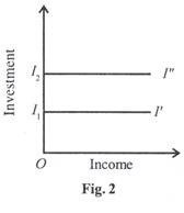
The upward shift of the curve to I2I” indicates an increased steady flow of investment at a constant rate OI2 at various levels of income. However, for purposes of income determination, the autonomous investment curve is superimposed on the С curve in a 45° line diagram.

3. Determinants of the Level of Investment:

The decision to invest in a new capital asset depends on whether the expected rate of return on the new investment is equal to or greater or less than the rate of interest to be paid on the funds needed to purchase this asset. It is only when the expected rate of return is higher than the interest rate that investment will be made in acquiring new capital assets.

In reality, there are three factors that are taken into consideration while making any investment decision. They are the cost of the capital asset, the expected rate of return from it during its lifetime, and the market rate of interest. Keynes sums up these factors in his concept of the marginal efficiency of capital (MEC).